How do you use Gaussian elimination to solve augmented matrix?
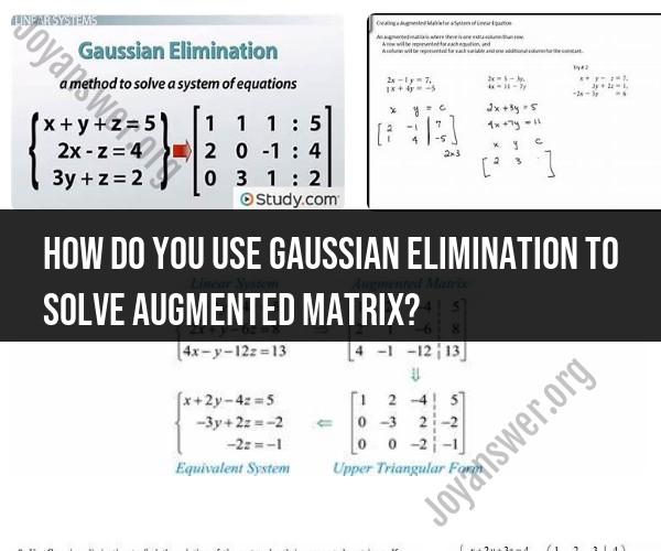
Gaussian elimination is a systematic method for solving systems of linear equations represented by augmented matrices. Here are step-by-step instructions on how to use Gaussian elimination to solve an augmented matrix:
Step 1: Set Up the Augmented Matrix
- Write down the system of linear equations in standard form, like this:
a₁x + b₁y + c₁z = d₁ a₂x + b₂y + c₂z = d₂ a₃x + b₃y + c₃z = d₃ - Create an augmented matrix by representing the coefficients of variables and constants on the right side of the equations in matrix form. The last column should contain the constants (d₁, d₂, d₃).
| a₁  b₁  c₁ | d₁ |
| a₂  b₂  c₂ | d₂ |
| a₃  b₃  c₃ | d₃ |
Step 2: Perform Row Operations
- Start with the first row (Row 1) and the first column (Column 1).
- Ensure that the leading coefficient (the first nonzero element) in Row 1 is 1. If it's not 1, divide the entire row by that element to make it 1.
- Use row operations to make all elements below the leading coefficient in Column 1 equal to 0. To do this, subtract multiples of Row 1 from the other rows.
- The augmented matrix should now have a leading 1 in Row 1, Column 1, and all elements below it should be zeros.
Step 3: Move to the Next Column
- Move to the second column (Column 2) and repeat the process. Ensure that the leading coefficient in Row 2 is 1, and use row operations to make all elements below it in Column 2 equal to 0.
- If Row 2 is already in the correct form, move on to Row 3 (if necessary).
Step 4: Continue the Process
- Repeat the process for each subsequent column, moving from left to right.
- Ensure that the leading coefficient in each row is 1 and use row operations to make all elements below it in the same column equal to 0.
- If necessary, swap rows to ensure that the row with the largest leading coefficient is at the top.
Step 5: Back-Substitution
- Once the augmented matrix is in row-echelon form (REF) or reduced row-echelon form (RREF), you can solve for the variables.
- Starting from the last row, work your way up, solving for each variable one at a time.
- For each row, use the known values of the variables you've already solved for to calculate the remaining variable(s).
- Continue until you have values for all variables.
Step 6: Check the Solution
- Substitute the found values back into the original equations to check if they satisfy all the equations.
- If the values satisfy all the equations, you have found the solution to the system of linear equations.
Gaussian elimination is a powerful method for solving systems of linear equations, but it can be complex for larger systems. It's important to carefully perform the row operations and maintain the integrity of the augmented matrix throughout the process.
Solving Linear Systems: Using Gaussian Elimination with Augmented Matrices
Gaussian elimination is a method for solving systems of linear equations by reducing the augmented matrix of the system to reduced row echelon form. The augmented matrix of a system of linear equations is a matrix that contains all of the coefficients of the system, as well as the constant terms.
To solve a system of linear equations using Gaussian elimination, we perform the following steps:
- Write the system of linear equations in augmented matrix form.
- Use elementary row operations to reduce the augmented matrix to reduced row echelon form.
- Solve the system of linear equations from the reduced row echelon form.
Example:
Solve the following system of linear equations using Gaussian elimination:
x + y + z = 6
2x - y + z = 3
-x + 2y - z = -2
Step 1: Write the system of linear equations in augmented matrix form.
[ 1 1 1 | 6 ]
[ 2 -1 1 | 3 ]
[ -1 2 -1 | -2 ]
Step 2: Use elementary row operations to reduce the augmented matrix to reduced row echelon form.
[ 1 1 1 | 6 ]
[ 0 -3 -1 | -9 ]
[ 0 0 0 | -17 ]
Step 3: Solve the system of linear equations from the reduced row echelon form.
The last row of the reduced row echelon form is the equation 0 = -17, which is impossible. Therefore, the system of linear equations has no solution.
Matrix Mathematics: Applying Gaussian Elimination to Augmented Matrices
Gaussian elimination can be understood in terms of matrix mathematics. The elementary row operations that are used to reduce the augmented matrix to reduced row echelon form can be represented by matrices. For example, the operation of multiplying a row by a constant can be represented by a diagonal matrix with the constant on the diagonal.
The following equation shows how Gaussian elimination can be represented in terms of matrix multiplication:
R = E * A
where:
- R is the reduced row echelon form of the augmented matrix A.
- E is a product of elementary matrices.
- A is the augmented matrix of the system of linear equations.
Step-by-Step Elimination: Solving Equations with Augmented Matrices
The following is a step-by-step guide for solving a system of linear equations using Gaussian elimination with augmented matrices:
- Write the system of linear equations in augmented matrix form.
- Eliminate the leading coefficient of the second row.
- Eliminate the leading coefficient of the third row.
- Back-substitute to solve for the variables.
Example:
Solve the following system of linear equations using Gaussian elimination with augmented matrices:
x + y + z = 6
2x - y + z = 3
-x + 2y - z = -2
Step 1: Write the system of linear equations in augmented matrix form.
[ 1 1 1 | 6 ]
[ 2 -1 1 | 3 ]
[ -1 2 -1 | -2 ]
Step 2: Eliminate the leading coefficient of the second row.
Subtracting 2 times the first row from the second row gives:
[ 1 1 1 | 6 ]
[ 0 -3 -1 | -9 ]
[ -1 2 -1 | -2 ]
Step 3: Eliminate the leading coefficient of the third row.
Adding the first row to the third row gives:
[ 1 1 1 | 6 ]
[ 0 -3 -1 | -9 ]
[ 0 3 0 | 4 ]
Step 4: Back-substitute to solve for the variables.
The third row of the augmented matrix gives us the equation 3y = 4, which means y = 4/3.
Substituting y = 4/3 into the second row of the augmented matrix, we get the equation -3x - 1 = -9, which means x = 2.
Substituting y = 4/3 and x = 2 into the first row of the augmented matrix, we get the equation 2 + 4/3 + z = 6, which means z = 6/3 - 6/3 = 0.
Therefore, the solution to the system of linear equations is x = 2, y = 4/3, and z = 0.
