What is the formula for macroeconomics?
Macroeconomics, the study of the economy as a whole, involves various fundamental concepts and equations. Here are some essential macroeconomic formulas:
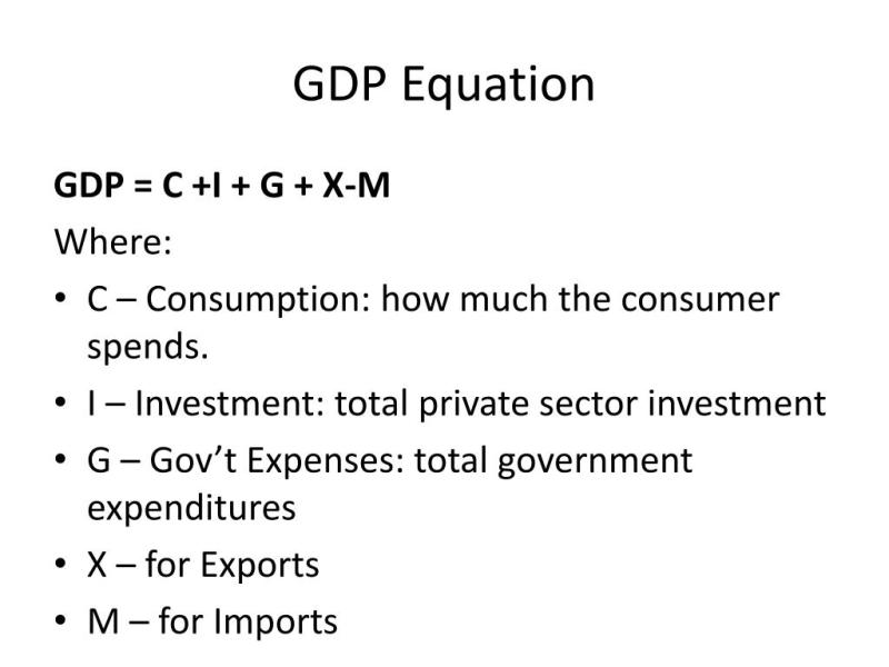
Gross Domestic Product (GDP):
- GDP measures the total economic output of a country.
Where:
- is consumption
- is investment
- is government spending
- is exports
- is imports
GDP Deflator:
- The GDP deflator is a measure of the overall price level in an economy.
Consumer Price Index (CPI):
- CPI measures the average change in prices paid by consumers for goods and services over time.
Unemployment Rate:
- The unemployment rate represents the percentage of the labor force that is unemployed and actively seeking employment.
Inflation Rate:
- Inflation measures the percentage change in the general price level of goods and services over time.
Multiplier Effect:
- The multiplier effect shows the change in GDP resulting from an initial change in spending.
Where is the marginal propensity to consume.
Phillips Curve:
- The Phillips Curve illustrates the trade-off between inflation and unemployment.
These formulas represent foundational concepts in macroeconomics. Keep in mind that the specific variables and equations used may vary depending on the economic model or theory being applied. Additionally, these equations provide a simplified view of complex economic relationships, and the real-world economy is influenced by various factors and dynamics.
What mathematical formulae constitute the foundation of macroeconomics?
While mathematical models and formulas play a significant role in macroeconomics, it's important to recognize that the field isn't solely built upon them. Macroeconomics draws upon various methodologies and theoretical frameworks to analyze and understand complex economic phenomena at the aggregate level, encompassing factors like inflation, unemployment, and economic growth.
However, some key mathematical formulas do serve as foundational pillars in macroeconomic analysis:
1. The Quantity Theory of Money (QTM):
This equation relates the money supply (M) to the price level (P), velocity of money (V), and real output (Y):
M * V = P * Y
The QTM suggests that changes in the money supply can influence inflation and economic activity. An increase in money supply (ceteris paribus) could lead to higher inflation or increased real output, depending on the velocity of money.
2. The IS-LM Model:
This model uses two equations to represent the equilibrium of the goods and services market (IS curve) and the money market (LM curve):
IS: Y = C(Y) + I(r) + GLM: M/P = L(r)
The IS curve represents the level of output at which aggregate demand (C + I + G) equals aggregate supply. The LM curve represents the equilibrium in the money market, where the supply of money (M/P) equals the demand for money (L(r)). The intersection of these curves determines the equilibrium level of output and interest rates.
3. The Solow-Swan Model:
This model explains long-run economic growth through the interplay of capital accumulation, population growth, and technological progress:
Y = K^α (AL)^{1-α}
Where:
- Y is output
- K is capital
- L is labor
- A is technological progress
- α is the capital share of income
The Solow-Swan model suggests that economic growth can be driven by capital accumulation, technological advancements, and population growth.
4. The Phillips Curve:
This relationship expresses a trade-off between inflation and unemployment:
π = f(u)
Where:
- π is the inflation rate
- u is the unemployment rate
The Phillips curve suggests that there may be a negative correlation between inflation and unemployment. Lower unemployment might be associated with higher inflation, and vice versa.
It's important to remember that these models are simplified representations of complex economic realities. They involve assumptions and limitations, and their interpretations should be made with caution. Macroeconomics utilizes a diverse set of tools and approaches, with mathematical formulas serving as valuable analytical instruments alongside theoretical frameworks, empirical data, and statistical analysis.